Worklowset over multiple time series (no panel)
Rafael Zambrano and Karina Bartolomé
Source:vignettes/workflowsets_multi_times.Rmd
workflowsets_multi_times.RmdAt a general level, this is the modeling scheme:

PS: An approach similar to that of our previous publication, Multiple Models Over Multiple Time Series: A Tidy Approach.
Workflowsets for multiple series 💡
🔹Considering the 4 series selected at the beginning. The first necessary step is to nest the series into a nested dataframe, where the first column is the state, and the second column is the nested_column (date and value).
data_states <-  USgas::us_residential %>% rename(value=y)

nested_data <- data_states %>%
  nest(nested_column=-state)
1️⃣Multiple workflows sets fit
The modeltime_wfs_multifit function from sknifedatar 📦 allows a 🌟 workflowset object to be fitted over multiple time series 🌟. In this function, the workflow_set object is the same as the one used before, since it contains the diferent model + recipes combinations.
Models 🚀
# prophet_xgboost
prophet_boost <-
  prophet_boost(mode = 'regression') %>% set_engine("prophet_xgboost")

# mars
mars <- mars( mode = 'regression') %>% set_engine('earth')
wfsets <- workflow_set(
  preproc = list(
    base                  = recipe_base,
    features              = recipe_date_features
  ),
  models  = list(
    M_prophet_boost     = prophet_boost,
    M_mars              = mars
  ),
  cross   = TRUE
)

wfsets
## # A workflow set/tibble: 4 x 4
## wflow_id info option result
## <chr> <list> <list> <list>
## 1 base_M_prophet_boost <tibble [1 × 4]> <opts[0]> <list [0]>
## 2 base_M_mars <tibble [1 × 4]> <opts[0]> <list [0]>
## 3 features_M_prophet_boost <tibble [1 × 4]> <opts[0]> <list [0]>
## 4 features_M_mars <tibble [1 × 4]> <opts[0]> <list [0]>
wfs_multifit <- modeltime_wfs_multifit(serie = nested_data %>% head(4),
                                       .prop = 0.9,
                                       .wfs  = wfsets)
👉 The fitted object is a list containing the fitted models (table_time) and the corresponding metrics for each model (models_accuracy).
wfs_multifit$table_time## # A tibble: 4 x 8
## state nested_column base_M_mars base_M_prophet_boost features_M_mars
## <chr> <list> <list> <list> <list>
## 1 Alabama <tibble [381 × 2]> <workflow> <workflow> <workflow>
## 2 Alaska <tibble [381 × 2]> <workflow> <workflow> <workflow>
## 3 Arizona <tibble [381 × 2]> <workflow> <workflow> <workflow>
## 4 Arkansas <tibble [381 × 2]> <workflow> <workflow> <workflow>
## # … with 3 more variables: features_M_prophet_boost <list>,
## # nested_model <list>, calibration <list>
wfs_multifit$models_accuracy## # A tibble: 16 x 11
## name_serie .model_id .model_names .model_desc .type mae mape mase smape
## <chr> <int> <chr> <chr> <chr> <dbl> <dbl> <dbl> <dbl>
## 1 Alabama 1 base_M_mars EARTH Test 1814. 123. 1.61 77.0
## 2 Alabama 2 base_M_proph… PROPHET Test 1064. 75.1 0.947 109.
## 3 Alabama 3 features_M_m… EARTH Test 860. 64.8 0.766 94.4
## 4 Alabama 4 features_M_p… PROPHET W/ … Test 1064. 75.1 0.947 109.
## 5 Alaska 1 base_M_mars EARTH Test 1732. 134. 4.11 145.
## 6 Alaska 2 base_M_proph… PROPHET Test 171. 15.8 0.406 14.3
## 7 Alaska 3 features_M_m… EARTH Test 815. 92.3 1.93 53.3
## 8 Alaska 4 features_M_p… PROPHET W/ … Test 191. 19.1 0.453 16.7
## 9 Arizona 1 base_M_mars EARTH Test 1842. 79.9 1.79 61.6
## 10 Arizona 2 base_M_proph… PROPHET Test 471. 13.1 0.457 14.1
## 11 Arizona 3 features_M_m… EARTH Test 520. 15.7 0.504 17.2
## 12 Arizona 4 features_M_p… PROPHET W/ … Test 471. 13.1 0.457 14.1
## 13 Arkansas 1 base_M_mars EARTH Test 2041. 169. 1.92 86.3
## 14 Arkansas 2 base_M_proph… PROPHET Test 605. 42.4 0.568 62.4
## 15 Arkansas 3 features_M_m… EARTH Test 417. 25.2 0.392 29.6
## 16 Arkansas 4 features_M_p… PROPHET W/ … Test 1026. 91.1 0.965 117.
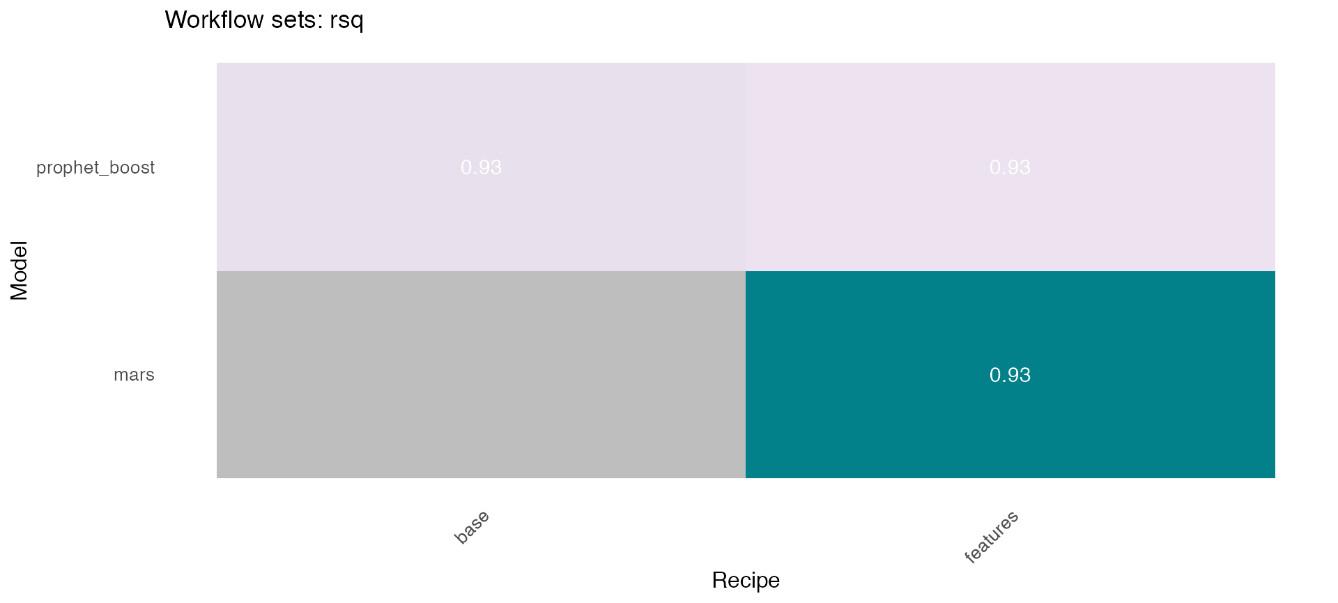
## # … with 2 more variables: rmse <dbl>, rsq <dbl>🔹 Using the models_accuracy table included in the wfs_multifit object, a heatmap can be generated for a specific metric for each series 🔍 . This is done using the modeltime_wfs_heatmap function presented above.
plots <- wfs_multifit$models_accuracy %>%
  dplyr::select(-.model_id) %>%
  dplyr::rename(.model_id=.model_names) %>%
  dplyr::mutate(.fit_model = '') %>%
  group_by(name_serie) %>%
  nest() %>%
  mutate(plot = map(data, ~ modeltime_wfs_heatmap(., metric = 'rsq',
                                                 low_color = '#ece2f0',
                                                 high_color = '#02818a'))) %>%
  ungroup()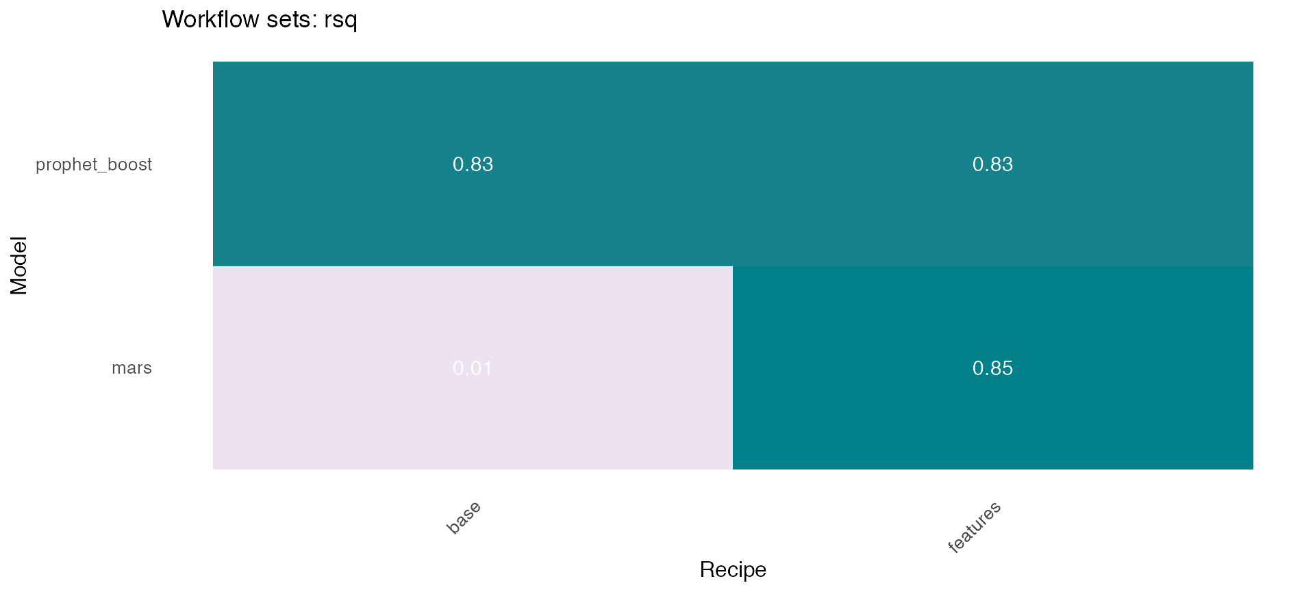
2️⃣Multiple forecast
Another function included in sknifedatar is modeltime_wfs_multiforecast, which generates 🧙 forecast of a workflow_set fitted object over multiple time series.
wfs_multiforecast <- modeltime_wfs_multiforecast(wfs_multifit$table_time,
                                                 .prop=0.9)
🔹The plot_modeltime_forecast function from modeltime is used to visualize each forecast, where the nested_forecast is unnnested before using the function. As it can be seen, many models did not perform well.
wfs_multiforecast %>%
      select(state, nested_forecast) %>%
      unnest(nested_forecast) %>%
      group_by(state) %>%
      plot_modeltime_forecast(
        .legend_max_width = 12,
        .facet_ncol = 2,
        .line_size = 0.5,
        .interactive = FALSE,
        .facet_scales = 'free_y',
.title='Proyecciones') 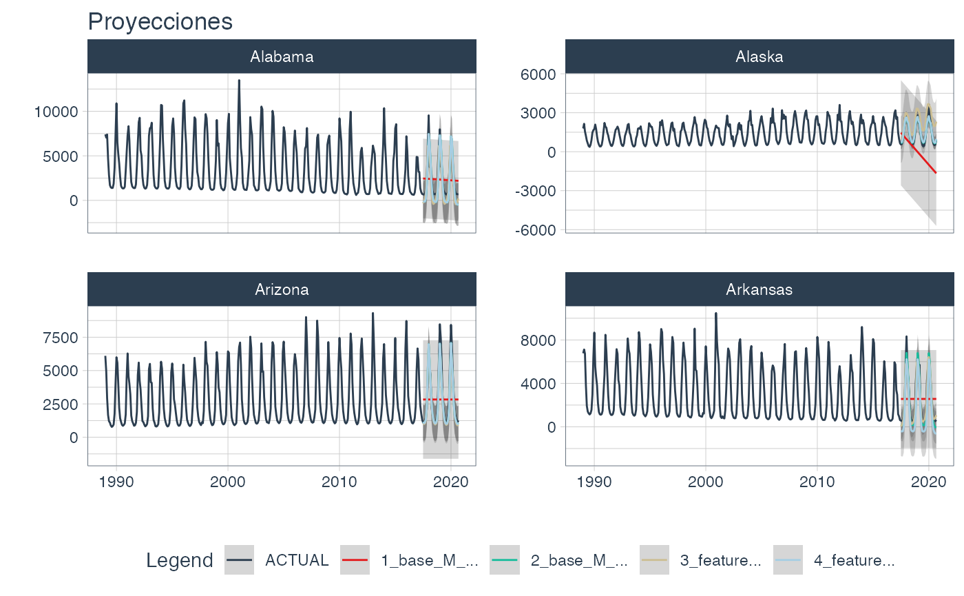
3️⃣ Best models
The modeltime_wfs_multibest 🏅 from sknifedatar obtains the best workflow/model for each time series based on a performance metric (one of ‘mae’, ‘mape’,‘mase’, ‘smape’,‘rmse’,‘rsq’).
wfs_bests<- modeltime_wfs_multibestmodel(
      .table = wfs_multiforecast,
      .metric = "rmse",
      .minimize = TRUE
    )
4️⃣Multiple refit
Now that we’ve selected the best model for each series, the modeltime_wfs_multirefit function is used in order to retrain a set of workflows on all the data (train and test) 👌
wfs_refit <- modeltime_wfs_multirefit(wfs_bests)5️⃣Final forecast
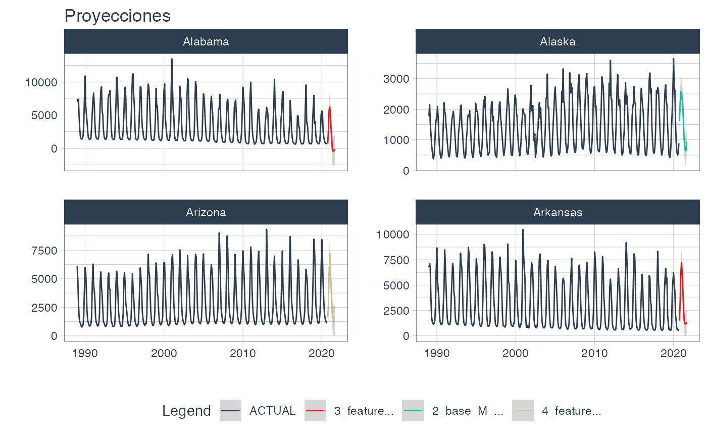
Finally, a new forecast is generated for the refitted object 🧙, resulting in 4 forecasts, one for each series. In this case, the modeltime_wfs_multiforecast is used with .h paramenter = ‘12 month’, giving a future forecast.
wfs_forecast <- modeltime_wfs_multiforecast(wfs_refit, .h = "12 month")

wfs_forecast %>%
      select(state, nested_forecast) %>%
      unnest(nested_forecast) %>%
      group_by(state) %>%
      plot_modeltime_forecast(
        .legend_max_width = 12,
        .facet_ncol = 2,
        .line_size = 0.5,
        .interactive = FALSE,
        .facet_scales = 'free_y',
        .title='Proyecciones')